This vignette demonstrates some of the use cases for curved text in ggplot.
Covid effects on life activities
After a design by George Stilabower
Data code block
df <- structure(list(xvals = rep(0:25, each = 13), yvals = c(
  9, 0, 0, 2, 0, 9, 10, 13, 0, 0, 0, 0, 0, 9, 0, 0, 2, 0, 9,
10, 13, 0, 0, 0, 0, 0, 9, 0, 1, 0, 4, 6, 10, 0, 13, 0, 0, 0,
0, 6, 3, 1, 0, 0, 10, 10, 0, 13, 0, 0, 0, 0, 6, 3, 1, 0, 0, 10,
10, 0, 13, 0, 0, 0, 0, 9, 0, 1, 0, 4, 6, 10, 0, 13, 0, 0, 0,
0, 9, 0, 1, 0, 4, 6, 10, 0, 13, 0, 0, 0, 0, 9, 0, 0, 2, 0, 9,
10, 0, 13, 0, 0, 0, 0, 9, 0, 0, 2, 0, 9, 10, 0, 13, 0, 0, 0,
0, 6, 3, 1, 0, 0, 10, 10, 0, 0, 13, 0, 0, 0, 3, 6, 1, 0, 0, 10,
10, 0, 0, 13, 0, 0, 0, 9, 0, 1, 0, 4, 6, 10, 0, 0, 13, 0, 0,
0, 9, 0, 0, 2, 0, 9, 10, 0, 0, 13, 0, 0, 0, 9, 0, 1, 0, 4, 6,
10, 0, 0, 13, 0, 0, 0, 6, 3, 1, 0, 0, 10, 10, 0, 0, 13, 0, 0,
0, 9, 0, 0, 2, 0, 9, 10, 0, 0, 13, 0, 0, 0, 9, 0, 0, 2, 0, 9,
10, 0, 0, 0, 13, 0, 0, 9, 0, 0, 2, 0, 9, 10, 0, 0, 0, 13, 0,
0, 9, 0, 0, 2, 0, 9, 10, 0, 0, 0, 0, 13, 0, 9, 0, 0, 2, 0, 9,
10, 0, 0, 0, 0, 13, 0, 9, 0, 1, 0, 4, 6, 10, 0, 0, 0, 0, 0, 13,
6, 3, 1, 0, 0, 10, 10, 0, 0, 0, 0, 0, 13, 9, 0, 0, 2, 0, 9, 10,
0, 0, 0, 0, 0, 13, 9, 0, 0, 2, 0, 9, 10, 0, 0, 0, 0, 0, 13, 9,
0, 0, 2, 0, 9, 10, 0, 0, 0, 0, 0, 13, 9, 0, 0, 2, 0, 9, 10, 0,
0, 0, 0, 0, 13)/20,
cols = structure(c(13L, 12L, 11L, 10L, 9L, 8L, 7L, 6L, 5L, 4L, 3L, 2L,
1L, 13L, 12L, 11L, 10L, 9L, 8L, 7L, 6L, 5L, 4L, 3L, 2L, 1L, 13L,
12L, 11L, 10L, 9L, 8L, 7L, 6L, 5L, 4L, 3L, 2L, 1L, 13L, 12L,
11L, 10L, 9L, 8L, 7L, 6L, 5L, 4L, 3L, 2L, 1L, 13L, 12L, 11L,
10L, 9L, 8L, 7L, 6L, 5L, 4L, 3L, 2L, 1L, 13L, 12L, 11L, 10L,
9L, 8L, 7L, 6L, 5L, 4L, 3L, 2L, 1L, 13L, 12L, 11L, 10L, 9L, 8L,
7L, 6L, 5L, 4L, 3L, 2L, 1L, 13L, 12L, 11L, 10L, 9L, 8L, 7L, 6L,
5L, 4L, 3L, 2L, 1L, 13L, 12L, 11L, 10L, 9L, 8L, 7L, 6L, 5L, 4L,
3L, 2L, 1L, 13L, 12L, 11L, 10L, 9L, 8L, 7L, 6L, 5L, 4L, 3L, 2L,
1L, 13L, 12L, 11L, 10L, 9L, 8L, 7L, 6L, 5L, 4L, 3L, 2L, 1L, 13L,
12L, 11L, 10L, 9L, 8L, 7L, 6L, 5L, 4L, 3L, 2L, 1L, 13L, 12L,
11L, 10L, 9L, 8L, 7L, 6L, 5L, 4L, 3L, 2L, 1L, 13L, 12L, 11L,
10L, 9L, 8L, 7L, 6L, 5L, 4L, 3L, 2L, 1L, 13L, 12L, 11L, 10L,
9L, 8L, 7L, 6L, 5L, 4L, 3L, 2L, 1L, 13L, 12L, 11L, 10L, 9L, 8L,
7L, 6L, 5L, 4L, 3L, 2L, 1L, 13L, 12L, 11L, 10L, 9L, 8L, 7L, 6L,
5L, 4L, 3L, 2L, 1L), .Label = c("Nesting Variable 6", "Nesting Variable 5",
"Nesting Variable 4", "Nesting Variable 3", "Nesting Variable 2",
"Nesting Variable 1", "blank", "mint", "green", "darkgray", "lightgray",
"red", "pink"), class = "factor")),
class = "data.frame", row.names = c(NA, -338L))


df_text <- data.frame(x = rep(0:25, each = 2)[-c(3:4)] + 0:1 -0.5,
                      y = 1.25, id = rep(0:25, each = 2)[-c(3:4)],
                      text = rep(c(
  "<strong>Total</strong>", "ipad", "Visits", "Parties", "Walks", "Home\nSchool", "Games",
  "Meals", "SPA", "Research", "HDU",
  "Meetings", "Admin", "Breaks", "Ward\nRounds", "Car", "Train", "Family", "Friends", "Github", "SO", "Docs", "Issues", "Debug",
  "Side\nProjects"), each = 2))

label1 <- paste("Family activities:",
                "These tended to increase",
                "during lockdown, but the",
                "types of activity",
                "changed.", sep = "\n")

label2 <- paste("Work activities:",
                "These were due",
                "directly to the",
                "medical effects",
                "of the pandemic.", sep = "\n")

label3 <- paste("Coding activities:",
                "These tended to increase",
                "during lockdown, but",
                "the focus changed",
                "depending on the",
                "needs of side",
                "projects.", sep = "\n")

fills <- rev(c("#e9cbc1", "#b54649", "gray90",
               "gray50", "#8ba55d", "#e2e4d6",
               "white", "#c3a891", "#37959d",
               "#5c7890", "#dcad3c", "#55a3b9",
               "#f39068"))

sep <- c(1.5, 8.5, 15.5, 17.5, 19.5)

sublabels <- data.frame(x = c(-0.25, 1.5, 2, 6, 9, 15, 16, 18, 18, 20, 20, 25),
                        y = 1.8,
                        id = c(0, 0, 1, 1, 2, 2, 3, 3, 4, 4, 5, 5),
                        z = rep(c("Sleeping", "Family", "Work",
                                  "Travel", "Social", "Coding"), each = 2))

covidpie <- list(df = df, df_text = df_text, fills = fills,
                 label1 = label1, label2 = label2, label3 = label3,
                 sep = sep, sublabels = sublabels)
ggplot(covidpie$df, aes(xvals, yvals)) +
  geom_col(width = 1.05, aes(fill = cols)) +
  geom_vline(colour = "white", xintercept = sep, size = 3) +
  geom_segment(data = data.frame(x = 0.5 + 1:24, y = 0, yend = 1),
               aes(x = x, y = 0, yend = 1, xend = x), colour = "white",
               inherit.aes = FALSE) +
  geom_textpath(data = covidpie$sublabels,
                mapping = aes(x, y, label = z, group = id), size = 3.8,
                upright = FALSE, text_only = TRUE, hjust = 0,
                color = "white", family = "Times New Roman") +

  geom_text(x = 32, y = -2, label = "Activities", check_overlap = TRUE,
            size = 7, family = "Times New Roman") +
  geom_text(x = 32, y = -1.4, label= "Changing time allocations\ndue to Covid",
            lineheight = 1, check_overlap = TRUE, family = "Times New Roman") +
  geom_textpath(data = covidpie$df_text, aes(x, y, label = text),
                upright = FALSE, size = 2, rich = TRUE, text_only = TRUE,
                halign = "left") +
  geom_text(x = 36.5, y = 1.8, label = covidpie$label1, hjust = 0,
            size = 2, check_overlap = TRUE, vjust = 1) +
  geom_text(x = 32.8, y = 0.75, label = covidpie$label2, vjust = 1, hjust = 0,
            size = 2, check_overlap = TRUE) +
  geom_text(x = 28.8, y = 1.04, label = covidpie$label3, hjust = 0,
            size = 2, check_overlap = TRUE, vjust = 1) +
  scale_y_continuous(limits = c(-2, 2.2)) +
  scale_fill_manual(values = covidpie$fills) +
  scale_x_continuous(expand = c(0.2, 1)) +
  coord_polar(start = -pi) +
  theme_void() +
  theme(legend.position = "none")
#> Warning: position_stack requires non-overlapping x intervals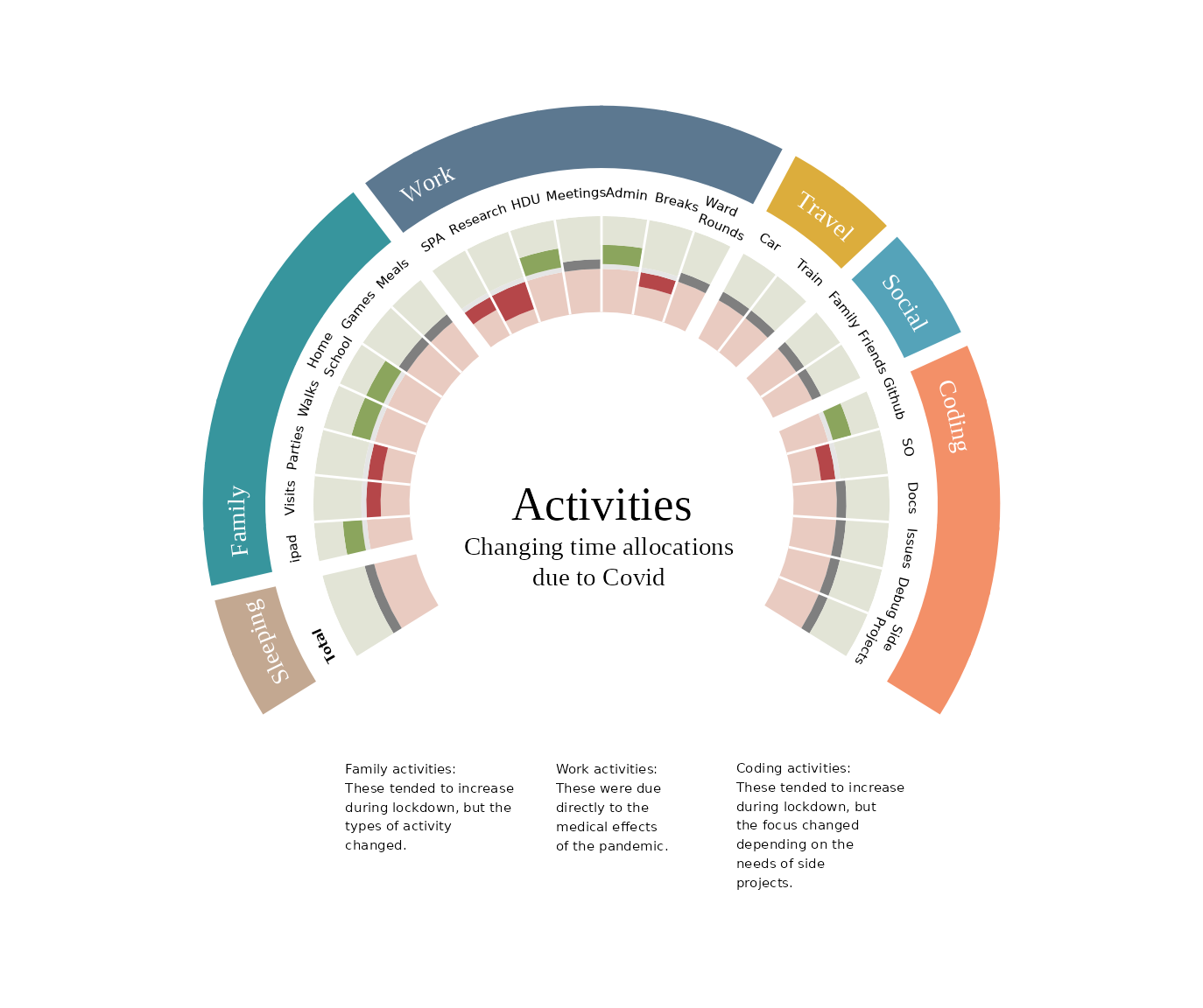
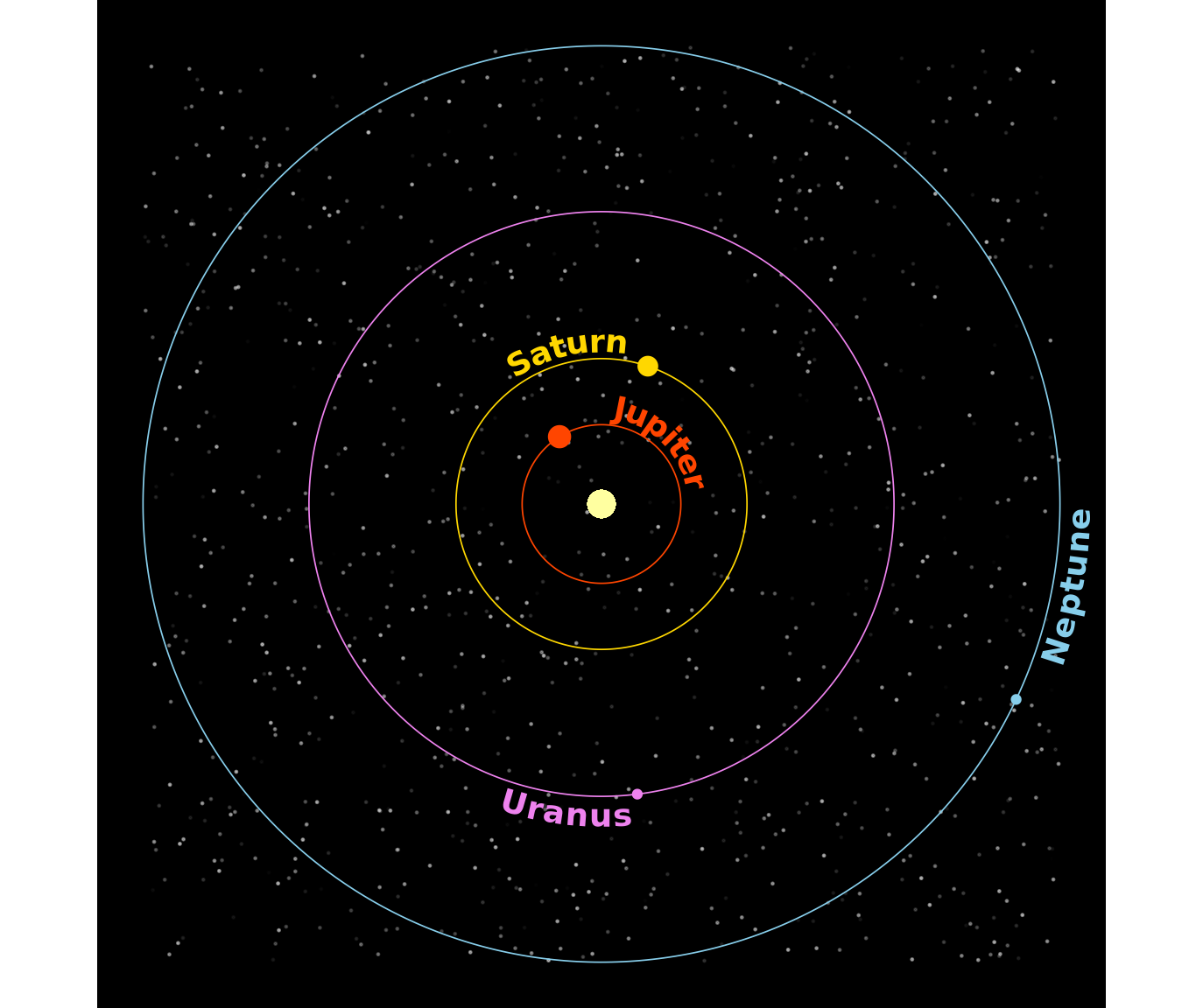
Planetary orbits
set.seed(1)
planets <- c("Jupiter", "Saturn", "Uranus", "Neptune")
t  <- seq(0, pi * 2, len = 500)
AU <- c(5.203, 9.539, 19.18, 30.06)

df <- data.frame(x = as.vector(outer(cos(t), AU)),
                 y = as.vector(outer(sin(t), AU)),
                 Planet = rep(planets, each = 500),
                 position = rep(c(0.75, 0.2, 0.4, 0.1)))

ggplot(df, aes(x, y, color = Planet)) +
  geom_point(inherit.aes = FALSE,
             data = data.frame(x = runif(1000, -30, 30),
                               y = runif(1000, -30, 30),
                               intens = runif(1000)/2),
             mapping = aes(x, y, alpha = intens), color = "white", size = 0.2) +
  geom_textpath(aes(label = Planet), linewidth = 0.3,
                hjust = rep(c(0, 0.25, 0.75, 1), each = 500),
                vjust = 1.1, size = 5, upright = TRUE, fontface = 2) +
  geom_point(data = df[c(170, 600, 1385, 1965),], size = c(4, 3.5, 1.5, 1.5)) +
  geom_point(x = 0, y = 0, size = 5, color = "#FFFFA0", inherit.aes = FALSE) +
  scale_alpha_identity() +
  scale_color_manual(values = c(Jupiter = "orangered",
                                Uranus ="violet",
                                Neptune = "skyblue",
                                Saturn = "gold")) +
  coord_equal() +
  theme_void() +
  theme(plot.background = element_rect(fill = "black"),
        legend.position = "none")